6 useful Google Sheets analysis formulas and techniques from my Twitch data analysis
I recently published a guide to analysing your Twitch data, from streamers watched to emotes used. This involved a lot of amazingly complicated Google Sheets formulas, enough to warrant a separate write-up. There are 6 extremely helpful formulas if you’re in a similar scenario, and should be somewhat interesting if not!
For reference, here is the spreadsheet all of these formulas are used in.
Dynamic row contents, with data lookup
The 3 columns in “Streamers watched” & “Players used” (title, count, minutes) are actually totally independent, with the main challenge coming from the dynamic data (e.g. streamer names) that might be there. I discovered =SORT(UNIQUE(Minutes!D2:D)) is an easy way to get an alphabetised list of all unique values in a range.
The “Count” column just counts the number of rows in the watch data features this player / streamer, e.g. COUNTIF(Minutes!$D$2:$D, E5). The “Minutes” column works the same, just with SUMIF.
One sneaky trick to avoid lots of 0s in the empty rows is some conditional formatting to set the text colour to white if the value is 0, which looks like an empty cell!
Largest values in a range
“Longest sessions” uses a technique I haven’t used before. By using LARGE we can get the top X value for a range, then find that value again, and fetch another cell in the row (using INDEX and MATCH). This might seem a convoluted way to fetch a top value but… that’s Google Sheets.
Filtering rows by timestamps
“Streams by year” was my first time messing around with dates in Google Sheets. All we need to do is use COUNTIF to count the rows whose timestamp meets both criteria: After or on the 1st Jan in the target year, and before 1st Jan the next year. This is combined with the count / sum logic from the player / streamer section to get totals.
Adding all numbers within text cells in a range
Here’s where the crazy formulas start! Getting the number of cheers messages was easy, just filter the sheet’s rows by type. The total bits donated were a bit trickier: my initial approach1 was finding all CheerX and adding them. This took a long time to get working, and I then realised you can send bits using words other than Cheer (e.g. ShowLove100). Oops!
My second approach was to just pull out all numbers in “Cheer” messages, and add them together. This has the potential to miscalculate (e.g. “Cheer100 10/10 stream” would count as 120 (100 + 10 + 10)), but it seems pretty accurate. However, this formula is a wild one:
- At the outer layer, we’re using some completely baffling
SUMandSPLITlogic to pull out all numerical values and add them together2. However, this only works for a single cell… - Putting a range into this formula works, we just need to dynamically define where the “cheer” rows appear in our Events. We need to do this twice, as the range appears twice in the formula.
- To get our starting point, we need to count the number of “chat” rows, then add 2:
COUNTIF(Events!$A$2:$A, "chat") + 2). This will be the first “cheer” row. - To get our finishing point, we need to use the same “chat” row count, and add the number of “cheer” rows (plus 1 due to zero indexing). So far, so good.
- Now the awkward bit. To combine these 2 into a range (e.g.
G100:G120), we need to useINDIRECT(to let us work with the cell reference as a string), andCONCATENATE(to combine our starting and ending point into a range).
Here’s how the process of building this formula looked, I hope this makes sense if I try to reuse it in a few months!
// Sum all numbers in a cell
=SUM(SPLIT(A1,CONCATENATE(SPLIT(A1,".0123456789"))))
// Sum all numbers in range
=SUM(SPLIT(A1:A10,CONCATENATE(SPLIT(A1:A10,".0123456789"))))
// Sum all numbers in range, with dynamic starting & ending point
=SUM(SPLIT(A<start point>:A<end point>,CONCATENATE(SPLIT(A<start point>:A<end point>,".0123456789"))))
// Sum all numbers in range, with dynamic starting & ending point, and string mangling
=SUM(SPLIT(CONCATENATE(INDIRECT("A" & <start point> & ":A" & <end point>)),CONCATENATE(SPLIT(CONCATENATE(INDIRECT("A" & <start point> & ":A" & <end point>)),".0123456789"))))
// Sum all numbers in range, with dynamic starting & ending point, and string mangling, and real start / end points, and full cell references
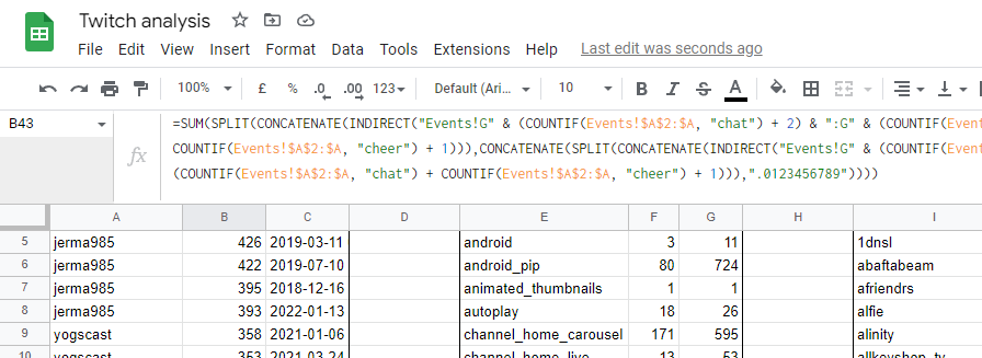
=SUM(SPLIT(CONCATENATE(INDIRECT("Events!G" & (COUNTIF(Events!$A$2:$A, "chat") + 2) & ":G" & (COUNTIF(Events!$A$2:$A, "chat") + COUNTIF(Events!$A$2:$A, "cheer") + 1))),CONCATENATE(SPLIT(CONCATENATE(INDIRECT("Events!G" & (COUNTIF(Events!$A$2:$A, "chat") + 2) & ":G" & (COUNTIF(Events!$A$2:$A, "chat") + COUNTIF(Events!$A$2:$A, "cheer") + 1))),".0123456789"))))
Counting occurrences of characters in range
To get the total chat messages (B40), I had to combine 2 bits of data:
- The total rows in “Events” that are chats or cheers:
COUNTIF(Events!A2:A, "chat") + COUNTIF(Events!A2:A, "cheers") - The number of times
;appears in these rows, as the raw data uses this when multiple messages are sent in a session. The number of these present are counted via some borderline magic usingArrayFormulaandSUBSTITUTE:3ArrayFormula(SUM(LEN(Events!G2:G))-SUM(LEN(SUBSTITUTE(Events!G2:G,";",""))))
Counting characters in a filtered range
Interestingly, chat characters required a totally different approach to chat messages. It’s also a formula I built entirely myself, whereas the rest are mostly other people’s work stuck together!
We can use our same dynamic range calculating & string mangling logic from “Cheers totals”, to give us our target range (all chat & cheer messages):
=INDIRECT("Events!G2:G" & (COUNTIF(Events!A2:A, "chat") + COUNTIF(Events!A2:A, "cheer") + 1))
This gives an array containing every chat or cheer message. We can then use ArrayFormula(LEN(...)) to convert this array of cells into an array of the character count in each cell. Finally, SUM(...)ing these give us… the total characters in all the filtered cells:
=SUM(ArrayFormula(LEN(INDIRECT("Events!G2:G" & (COUNTIF(Events!A2:A, "chat") + COUNTIF(Events!A2:A, "cheer") + 1)))))